Same model, same learning rate, and only the mean and spread of the inputs change, yet training slows down or diverges. Deep learning data distribution and the learning rate, explained with E[x²].
Sometimes the model code is the same, the learning rate is the same, and training still fails after you swap the data. You read the code again and find nothing wrong. The cause is on the data side. This part shows, with experiments, how the deep learning data distribution, that is, the mean and spread of the inputs, changes training.
Series guide: See all 11 parts and what is already published in the Deep Learning Math in C++ roadmap. This part reuses the multiplier
f = 1 − 2x²αfrom part 3: learning rate.
The short answer
As part 3 showed, each update multiplies the remaining distance by 1 − 2x²α, so the size of x² decides whether training is stable. If x has mean μ and standard deviation σ, the average of x² is E[x²] = μ² + σ² (this holds for any distribution, not just the normal distribution). So a larger spread, or a mean further from 0 in either direction, makes the same learning rate diverge, and a good learning rate shrinks to roughly 1/(2·E[x²]).
What this post answers
- Why changing only the data distribution changes the result at the same learning rate
- How the standard deviation and the mean each affect training
- Why inputs with mean +15 and mean −15 are equally dangerous
- How to estimate a learning rate from the data distribution
New terms in this part
| Term | Meaning |
|---|---|
| Distribution | Where data values sit and how they are spread |
Normal distribution N(μ, σ²) | The bell-shaped distribution centered on the mean μ; σ is the standard deviation |
| Mean (μ) | The center of the values |
| Standard deviation (σ) | How widely values spread around the mean |
E[x²] | The average (expected value) of x². For any distribution with mean μ and standard deviation σ it equals μ² + σ² |
| Synthetic data | Data generated from a known answer, used to check that training finds it |
Setup: data whose answer is 1
This time the answer is y = x, that is, θ = 1. The model is ŷ = θx as in part 1, starting from θ = 0.1. The only thing that changes is the distribution x is drawn from.
With y = x, the derivation from part 3 gives, for one update:
θ_new − 1 = (1 − 2αx²)(θ − 1)Only the answer changed from 3 to 1; the multiplier is the same. Because the multiplier contains x², the distribution x comes from decides the multiplier.
Why the average of x² is μ² + σ²
Write x as “the mean μ plus a deviation d”. Then x² = μ² + 2μd + d². The deviation d averages to 0, so the middle term 2μd averages to 0, and the average of d² is the variance σ².
E[x²] = μ² + σ²Two things follow:
- When σ grows: occasionally a very large |x| appears, its x² is large, and that sample makes one update jump.
- When |μ| grows: every x is far from 0, so x² is always large. μ enters squared, so +15 and −15 are equally dangerous.
Checking it in C++ and Python
C++ and Python random generators produce different values even with the same seed (see part 1), so instead of random numbers we fix 10 values chosen to look like a standard normal sample. Applying x = μ + σ × z to these 10 values mimics any distribution, and both languages print exactly the same output.
The learning rate is fixed at 0.008, and the 10 samples are trained for 10 epochs (100 updates). The epoch f column is part 3’s “product of the per-sample multipliers over one epoch”. If its absolute value is below 1 training converges; above 1 it diverges.
C++ (C++17, no external libraries)
#include <cstdio>
#include <utility>
#include <vector>

double Train(const std::vector<double>& xs, double lr, int epochs, double th = 0.1) {
    for (int epoch = 0; epoch < epochs; ++epoch)
        for (double x : xs) {
            const double y = x;                          // the answer is y = x, so θ = 1
            th = th + 2.0 * x * lr * (y - th * x);       // part 2 update rule
        }
    return th;
}

int main() {
    // 10 fixed values that look like a standard normal sample (mean 0, std about 0.94)
    const std::vector<double> z = {-1.6, -1.1, -0.7, -0.4, -0.1, 0.1, 0.4, 0.7, 1.1, 1.6};
    const double lr = 0.008;
    const std::vector<std::pair<double, double>> settings = {
        {0, 1}, {0, 2}, {0, 5}, {0, 10}, {0, 15}, {5, 1}, {15, 1}, {-15, 1}};

    for (const auto& [mean, std_dev] : settings) {
        std::vector<double> xs;
        for (double v : z) xs.push_back(mean + std_dev * v);   // mimic x ~ N(mean, std^2)

        double ex2 = 0.0, epoch_f = 1.0;
        for (double x : xs) {
            ex2 += x * x;                                // sum for the average of x^2
            epoch_f *= 1.0 - 2.0 * lr * x * x;           // part 3 multiplier, multiplied over one epoch
        }
        ex2 /= xs.size();

        char label[32];
        std::snprintf(label, sizeof(label), "N(%g,%g^2)", mean, std_dev);
        std::printf("%-11sE[x^2]=%7.2f  epoch f=%+10.3g  th=%.6gn", label, ex2, epoch_f,
                    Train(xs, lr, 10));
    }
}
Python (standard library only)
# 10 fixed values that look like a standard normal sample (mean 0, std about 0.94)
z = [-1.6, -1.1, -0.7, -0.4, -0.1, 0.1, 0.4, 0.7, 1.1, 1.6]

def train(xs, lr, epochs, th=0.1):
    for _ in range(epochs):
        for x in xs:
            y = x                                  # the answer is y = x, so θ = 1
            th = th + 2 * x * lr * (y - th * x)    # part 2 update rule
    return th

lr = 0.008
for mean, std in [(0, 1), (0, 2), (0, 5), (0, 10), (0, 15), (5, 1), (15, 1), (-15, 1)]:
    xs = [mean + std * v for v in z]               # mimic x ~ N(mean, std^2)
    ex2 = sum(x * x for x in xs) / len(xs)         # average of x^2
    epoch_f = 1.0
    for x in xs:
        epoch_f *= 1 - 2 * lr * x * x              # part 3 multiplier, multiplied over one epoch
    th = train(xs, lr, 10)
    print(f"N({mean},{std}^2)".ljust(11) + f"E[x^2]={ex2:7.2f}  epoch f={epoch_f:+10.3g}  th={th:.6g}")
Output
N(0,1^2)   E[x^2]=   0.89  epoch f=    +0.866  th=0.786622
N(0,2^2)   E[x^2]=   3.54  epoch f=    +0.546  th=0.997871
N(0,5^2)   E[x^2]=  22.15  epoch f= +8.62e-05  th=1
N(0,10^2)  E[x^2]=  88.60  epoch f=     +0.21  th=1
N(0,15^2)  E[x^2]= 199.35  epoch f=     +74.1  th=-4.51456e+18
N(5,1^2)   E[x^2]=  25.89  epoch f=  +0.00324  th=1
N(15,1^2)  E[x^2]= 225.89  epoch f= +1.28e+04  th=-1.05987e+41
N(-15,1^2) E[x^2]= 225.89  epoch f= +1.28e+04  th=-1.05987e+41
Reading the results
Growing the standard deviation: slow → fast → divergent
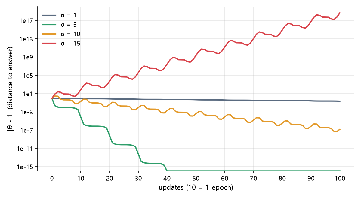
- σ = 1:
E[x²]is only 0.89, so each update moves very little. After 100 updates θ is at 0.786622, far from 1. The learning rate 0.008 is too small for this data. - σ = 5: the fastest. The distance shrinks about ten-thousandfold per epoch, and after 40 updates θ is indistinguishable from 1 in floating point.
- σ = 10: it converges, but the curve bumps within each epoch. The largest x (16) has a per-sample multiplier of −3.1, which momentarily increases the distance before the other samples shrink it again.
- σ = 15: the other samples can no longer absorb the jumps caused by large x; the distance grows 74-fold per epoch and training diverges.
The same learning rate 0.008 is too small for σ = 1 and too large for σ = 15. Whether a learning rate is “right” depends on the data distribution.
Moving the mean away from 0
Mean 5 (E[x²] = 25.89) converges quickly, but mean 15 (E[x²] = 225.89) diverges. And means +15 and −15 give exactly the same result. In the update rule, x enters the multiplier only as x², so flipping the sign does not change how training unfolds (the fixed values z are symmetric around 0, so both datasets have the same x² values in a different order). “The data are negative, so it should be fine” does not hold.
Note also that mean 15 diverged with a standard deviation of only 1. The values are tightly packed, but being far from 0 makes every sample’s x² large.
Random data lead to the same conclusion
The experiment above used fixed values, but the original C++ example drew 100 random samples and trained 1 epoch at learning rate 0.008. The table shows the last θ recorded in the training log.
| Distribution | Last θ | Result |
|---|---|---|
| N(0, 1) | 0.773985 | slow |
| N(0, 5²) | 1 | converged |
| N(0, 10²) | 1 | converged |
| N(0, 15²) | −1.39732e+13 | diverged |
| N(15, 1) | 2.08467e+41 | diverged |
| N(−15, 1) | 8.61398e+39 | diverged |
With random samples the numbers for +15 and −15 differ, but both diverge.
The same example also tried 12 candidate learning rates (0.0001 to 0.5) for each distribution and recorded the learning rate that got θ within 0.001 of 1 and kept it there fastest.
| Distribution | E[x²] | Fastest learning rate | Theory 1/(2·E[x²]) |
|---|---|---|---|
| N(0, 1) | 1 | 0.2 | 0.5 |
| N(0, 3²) | 9 | 0.02 | 0.056 |
| N(−3, 2²) | 13 | 0.05 | 0.038 |
| N(5, 1) | 26 | 0.02 | 0.019 |
| N(10, 5²) | 125 | 0.002 | 0.004 |
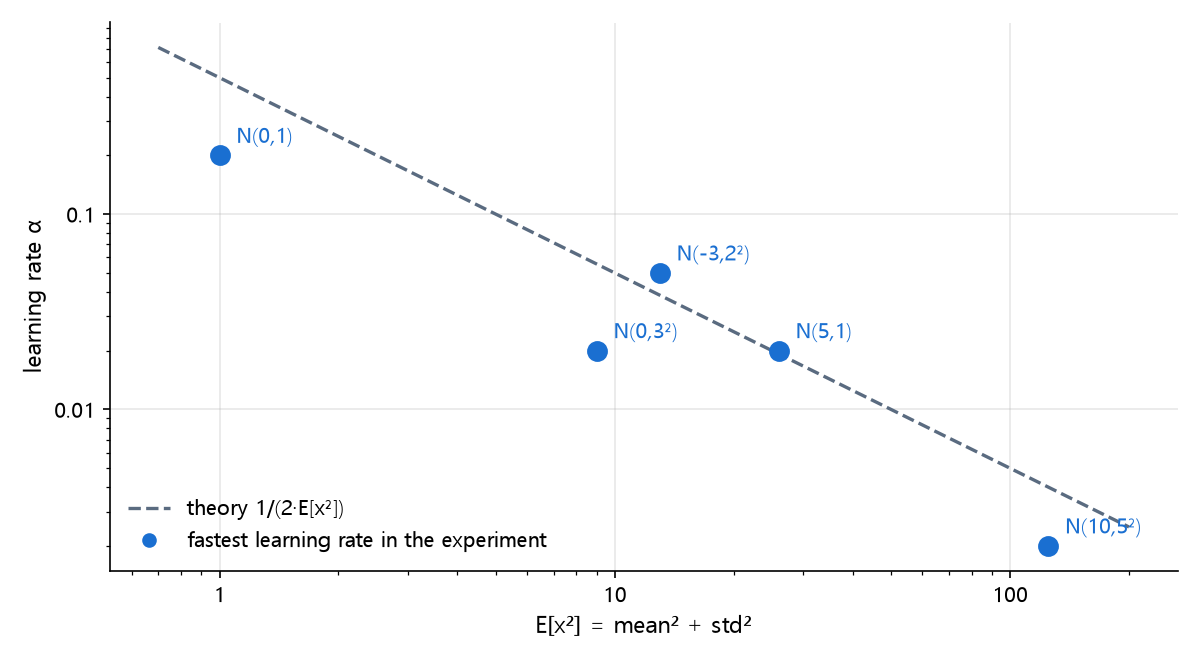
The points do not sit exactly on the theoretical line, because the candidate learning rates are coarse and the actual x² values of a sample are not captured by one average. The trend is still clear: when E[x²] grows tenfold, a good learning rate shrinks roughly tenfold.
What to remember in practice
- Check the mean and standard deviation of the inputs before training. It takes a few lines and tells you where to start the learning rate search.
- Use
1/(2·E[x²])as a starting point. It is not exact, but it has the right order of magnitude; scale up or down from there. - With several inputs, the largest one limits the learning rate. If you feed height (around 170) and eyesight (around 1) together, the learning rate must be small enough for height, and the eyesight weight learns very slowly.
- Changing the distribution is the real fix. Instead of tuning the learning rate per dataset, rescale the inputs to mean 0 and standard deviation about 1, and the same learning rate trains stably. That is feature scaling, covered in part 10.
Common sources of confusion
“Tightly packed values are safe” can be wrong
Data with mean 15 and standard deviation 1 are tightly packed, yet they diverged. What matters is not the spread σ alone but the whole of μ² + σ².
Slow training can also come from the distribution
With σ = 1, θ stalled at 0.79 because the learning rate was too small for this data. Before concluding that “the model cannot learn”, check the relationship between the learning rate and the input size.
The formula here is exact only for one-dimensional linear regression
1/(2·E[x²]) was derived for this model. You cannot plug it into a complex neural network, but the principle, larger inputs need a smaller learning rate, still applies.
Deep learning data distribution in summary
- The update multiplier
1 − 2αx²contains x², so the input distribution decides how stable training is. E[x²] = μ² + σ², so a larger spread or a mean further from 0 makes the same learning rate diverge.- The sign of the mean does not matter; +15 and −15 are equally dangerous.
- A good learning rate shrinks roughly like
1/(2·E[x²]), and the real fix is feature scaling, which brings inputs to a fixed size.
The next part compares updating after every sample (SGD), updating once from all samples (batch), and the middle ground (mini-batch).
Try it yourself
- Lower the learning rate from 0.008 to 0.002 and run again. For
N(0,15²),E[x²]is about 200, so the theory value is1/(2×200) = 0.0025. At 0.002, close to it, the data that diverged now converge to 1. - Keep the standard deviation at 1 and raise only the mean, 5, 6, 7, …, until the absolute value of
epoch ffirst exceeds 1. With this data and learning rate 0.008, means up to 11 converge and 12 diverges.