Train a one-parameter linear regression model in C++ and Python and watch the predict, measure, update loop of deep learning happen with real numbers.
You decide to learn deep learning, open the first chapter, and find a straight line instead of a neural network. It is easy to feel let down, or to wonder why you are back at y = ax + b. But when you implement deep learning linear regression yourself in C++, you find that this simple line already contains almost the entire skeleton of how deep learning trains.
Series guide: See all 11 parts and what is already published in the Deep Learning Math in C++ roadmap.
The short answer
Deep learning starts with linear regression because its training loop, predict → measure the error → compute the gradient → update the parameter, is the same loop a huge neural network uses. With only one parameter you can follow every step with your own eyes, and because you know the right answer in advance, you can check whether training actually worked.
What this post answers
- What “training” means as an actual computation
- Three reasons linear regression is the right starting point
- How θ really changes when trained in C++
- Why training ends at 2.97 instead of the true value 3
Key deep learning terms first
These terms appear throughout this post and the whole series. The right column shows what each term refers to in this post’s experiment.
| Term | Meaning | In this experiment |
|---|---|---|
| Model | A formula that turns an input into a prediction | ŷ = θx |
| Parameter | A value inside the model that training changes. “Training” means changing parameters | the single θ |
| Weight | A parameter multiplied by an input; how strongly the input affects the result | θ (the slope) |
| Bias | A parameter added regardless of the input; the intercept of a line | none (added in part 7 as ŷ = θ1·x + θ0) |
| Sample | One input–answer pair (x, y) | 100 samples |
| Prediction | The model’s answer, written ŷ (“y hat”) | θ × x |
| Loss | How wrong the prediction is for one sample | (y − ŷ)² |
| Cost | The average loss over several samples | covered in part 6 |
| Gradient | How much, and in which direction, the loss changes when a parameter changes; found by differentiation | −2x(y − ŷ) |
| Gradient descent | Reducing the loss by moving parameters a little against the gradient | the θ update rule |
| Learning rate | How large one update step is; written α or lr | 0.001 |
| Update (step) | Changing the parameters once; also called an iteration | 5,000 in total |
| Epoch | One full pass over all the data | 50 epochs (1 epoch = 100 updates) |
| Batch | The samples used together for one update | one sample at a time (compared in part 6) |
Two notes:
- Weight and bias: in neural networks, people often call all weights and biases together “parameters” or just “weights”. The θ here multiplies the input x, so it is a weight. The word bias is shared with the statistical term for systematic skew, but inside a model it simply means the constant term that is added.
- Epochs and updates: with 100 samples and one update per sample, one epoch is 100 updates, so 50 epochs are 5,000 updates. The same training looks different depending on whether a chart’s x-axis is updates or epochs, so always check the unit.
A deep learning linear regression experiment: the answer is 3
First we build a problem whose answer we know. We draw 100 random inputs x and make the targets y by adding a little noise to 3x.
- Data:
y = 3x + 0.5 × (standard normal noise), 100 samples - Model:
ŷ = θx(a single slope θ, no intercept) - Start:
θ = 0.1(deliberately far from 3)
The model does not know the answer is 3. The question is whether, from the data alone, it can move θ close to 3 by itself.
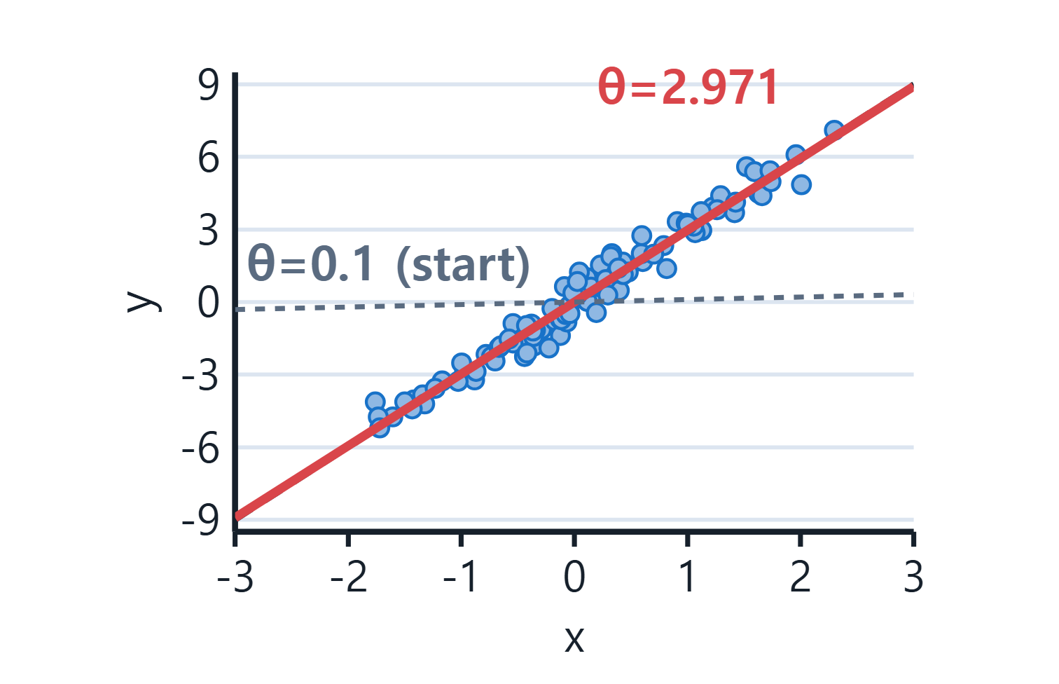
The starting line (dashed, θ=0.1) is almost flat and explains nothing. The trained line (red, θ=2.971) runs right through the middle of the data. This post is about what happens while the dashed line turns into the red one.
Training is these four steps, repeated
Each time a sample (x, y) comes in, the model does four things.
- Predict: compute
ŷ = θxwith the current θ. - Measure the error:
loss = (y − ŷ)². Squaring makes large mistakes count much more. - Compute the gradient: use the derivative to see whether making θ a little bigger increases or decreases the loss.
- Update: move θ a little in the direction that reduces the loss.
Put together, the rule for changing θ becomes a single line.
θ ← θ + 2 · α · x · (y − ŷ)α (the learning rate) sets how big each move is. Part 2 (deriving the gradient descent update rule) shows where this line comes from. For now it is enough to read it as “correct θ in proportion to the error (y − ŷ) and the input size (x)”.
The same loop in C++ and Python
Here are the four steps as code, side by side. Each program has a data part and a training part, and the core of the training part is three lines in both languages.
C++ (C++17, no external libraries)
#include <iostream>
#include <random>
#include <vector>

int main() {
    // Make the data: y = 3x + 0.5 * noise
    std::mt19937 rng(0);                                   // fixed random seed
    std::normal_distribution<double> normal(0.0, 1.0);
    const std::size_t n_sample = 100;
    std::vector<double> x_data(n_sample), y_data(n_sample);
    for (auto& x : x_data) x = normal(rng);                // x ~ N(0, 1)
    for (std::size_t i = 0; i < n_sample; ++i)
        y_data[i] = 3.0 * x_data[i] + 0.5 * normal(rng);   // y = 3x + noise

    // Train
    double th = 0.1;                                       // start far from 3
    const double lr = 0.001;                               // learning rate
    for (std::size_t epoch = 0; epoch < 50; ++epoch) {     // 50 passes over the data
        for (std::size_t i = 0; i < n_sample; ++i) {
            const double x = x_data[i], y = y_data[i];
            const double pred = th * x;                    // 1) predict
            [[maybe_unused]] const double loss = (y - pred) * (y - pred);  // 2) error
            th = th + 2.0 * x * lr * (y - pred);           // 3)+4) gradient and update
        }
    }
    std::cout << "learned th = " << th << 'n';
}
Python (NumPy)
import numpy as np

# Make the data: y = 3x + 0.5 * noise
np.random.seed(0)                                       # fixed random seed
n_sample = 100
x_data = np.random.randn(n_sample)                      # x ~ N(0, 1)
y_data = 3 * x_data + 0.5 * np.random.randn(n_sample)   # y = 3x + noise

# Train
th = 0.1                                                # start far from 3
lr = 0.001                                              # learning rate
for epoch in range(50):                                 # 50 passes over the data
    for x, y in zip(x_data, y_data):
        pred = th * x                                   # 1) predict
        loss = (y - pred) ** 2                          # 2) error
        th = th + 2 * x * lr * (y - pred)               # 3)+4) gradient and update

print("learned th =", th)
Side by side, the training parts match line for line; only the syntax differs. There are no library calls, just multiplication, subtraction, and addition. A huge neural network has the same loop. The differences are that it has billions of parameters instead of one, and it computes gradients with backpropagation instead of a hand-derived formula. In the C++ code, [[maybe_unused]] marks that loss is computed only to show the step, which stops the compiler’s “unused variable” warning.
The real difference is in making the data. Python fills an array with one call to np.random.randn, while C++ needs a random engine (std::mt19937) and a distribution (std::normal_distribution) and fills the array in a loop. The two languages also use different random algorithms, so the same seed 0 produces different data.
| Run | Data | Learned θ |
|---|---|---|
| C++ | C++ random numbers (mt19937, seed 0) | 2.97091 |
| Python | NumPy random numbers (seed 0) | 3.06161 |
| Python | Reads the data C++ generated | 2.97091 |
Python’s 3.06161 is not wrong; it is the result of training on 100 different samples. The least-squares answer for that data is 3.05955, and training went right next to it. When Python is given the data C++ generated, it learns exactly 2.97091. Different languages, same training computation.
The results and charts below use the C++ run.
What the run shows
100 samples, 50 epochs, 5,000 updates in total:
| Item | Value |
|---|---|
| Starting θ | 0.1 |
| Learned θ | 2.97091 |
| True value | 3 |
| First update with |θ − 3| < 0.1 | update 2,100 (epoch 22) |
| Mean loss in the last epoch | 0.2622 |
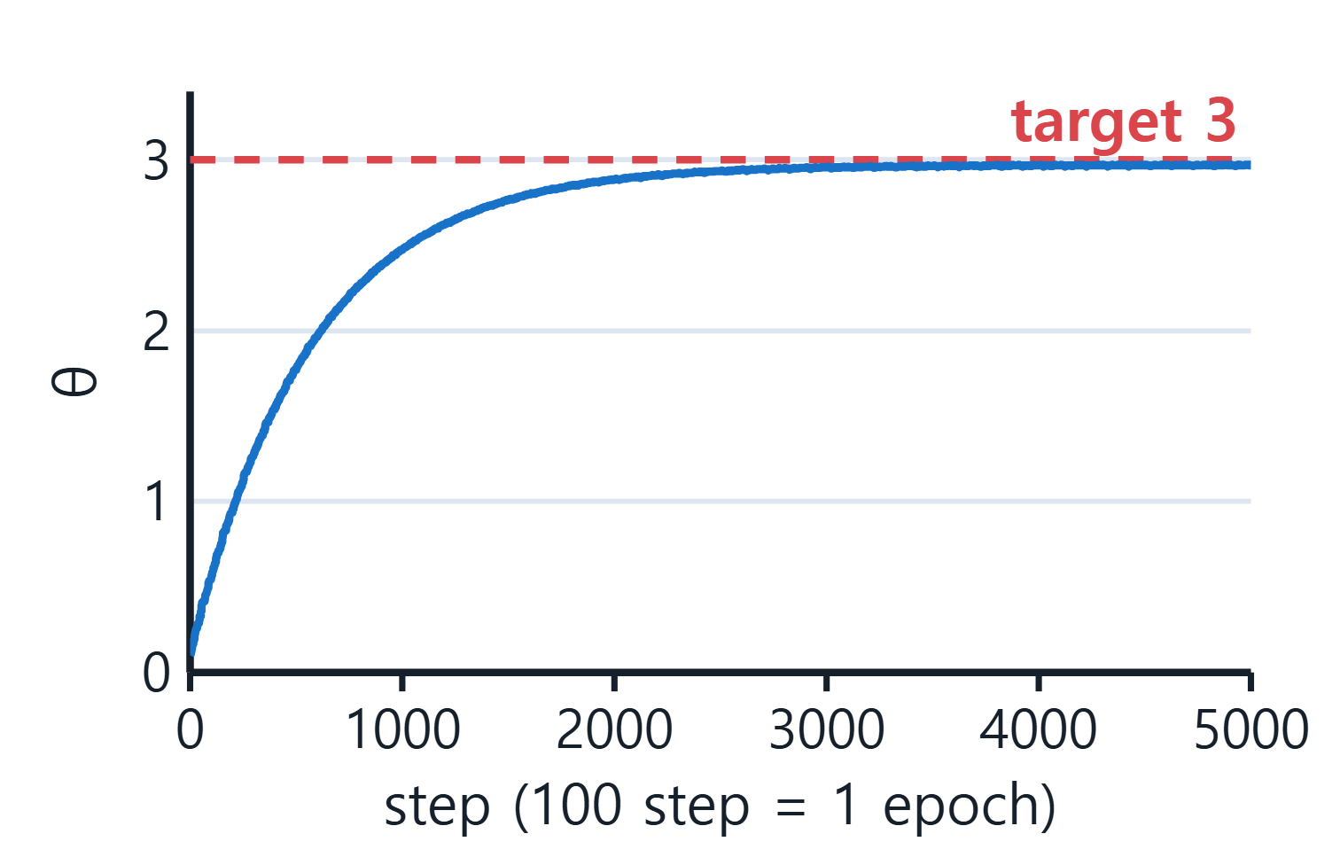
θ climbs fast at first and slows down as it approaches 3. Far from the answer, the error (y − ŷ) is large, so each correction is large; near the answer, the error is small, so corrections shrink. Nobody told the model to slow down. The update rule itself behaves that way.
Reason 1. It shows the training loop of a neural network at its smallest
The predict → error → gradient → update loop in the code above is the same structure most deep learning models use. Image classifiers and language models also repeat “predict with the current parameters, measure how wrong that was, move the parameters slightly so it is less wrong” a very large number of times.
Linear regression keeps that loop and shrinks only the model part to its simplest form. Once the loop is clear here, a more complex model reads as “the model changed, the training did not”.
Reason 2. The error landscape is a parabola you can see
For a single sample, the loss is a quadratic function of θ: a parabola. It has one bottom, so there is never any doubt about which way to go.
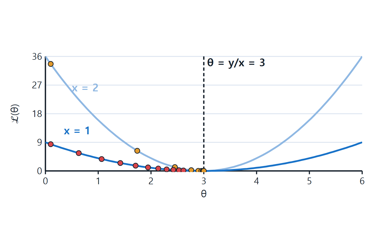
The two parabolas are the loss of one sample on y = 3x, with x=1 and x=2. Both touch zero loss at θ = 3. The red dots (x=1) and orange dots (x=2) mark θ every 10 updates with learning rate 0.01. The steeper x=2 side reaches the bottom much faster: getting within 0.01 of 3 took 281 updates for x=1 but only 68 for x=2.
Here are the first four updates by hand (x = 1, y = 3, learning rate 0.01):
| Update | θ | Prediction ŷ | Loss | Gradient | Next θ |
|---|---|---|---|---|---|
| 0 | 0.1000 | 0.1000 | 8.4100 | −5.8000 | 0.1580 |
| 1 | 0.1580 | 0.1580 | 8.0770 | −5.6840 | 0.2148 |
| 2 | 0.2148 | 0.2148 | 7.7571 | −5.5703 | 0.2705 |
| 3 | 0.2705 | 0.2705 | 7.4499 | −5.4589 | 0.3251 |
A negative gradient means “increasing θ lowers the loss”, so θ grows. And the remaining distance 3 − θ shrinks by exactly 0.98 each time. That 0.98 decides both the speed of training and whether it blows up, and it comes back in part 3 (learning rate).
You cannot draw this landscape for a model with billions of parameters. With linear regression you can, so “walking down the slope” stops being a metaphor and becomes a picture.
Reason 3. You know the answer, so you can check it
In real problems you never know the right parameters. When training goes badly, it is hard to tell whether the code is wrong or the data is hard. This experiment was built with the answer 3, so the result can be checked directly.
Yet the learned θ was 2.97091, not 3. Did training fail?
The slope that fits this exact data best (the least-squares solution, Σxy / Σx²) is 2.96927. With noise mixed into only 100 samples, “the slope that fits this data best” is a little below 3, and training went right to it. The gap from 3 comes from the noise in the data, not from a training mistake.
Having a known answer to compare against is what lets you say “training worked” with numbers. That is one more reason linear regression is a good first step.
Three results that are easy to misread
A loss that never reaches zero is not a failure
The mean loss in the last epoch was 0.2622. The noise added to the data has variance 0.5² = 0.25, so no amount of training can push the loss much below that. “The loss stopped going down” does not mean “training failed”.
θ keeps wobbling after training
Because this experiment updates θ after every sample, θ kept moving between 2.9627 and 2.9730 during the last epoch. Each sample pulls in a slightly different direction. Reducing that wobble is the topic of part 6 (batch, SGD, and mini-batch).
A bigger learning rate is not always faster
The learning rate 0.001 is safe but slow: reaching within 0.1 of 3 took 22 epochs. A larger learning rate is faster, but past a certain point θ overshoots the bottom and moves away. Part 3 finds that boundary with real numbers.
Deep learning linear regression in summary
- Deep learning training is a loop of predict → error → gradient → update, and linear regression shows that loop at its smallest.
- With one parameter and a parabola-shaped error landscape, you can follow training to the end with charts and numbers.
- Starting from a known answer lets you verify the result, including the fact that 2.97 is “the value that fits this data best”.
The next part derives the update rule θ ← θ + 2αx(y − ŷ), which we took on trust here, with a single derivative.
Try it yourself
If you can run the code, change just two things.
- Start from
θ = 6.0instead ofθ = 0.1. Check whether θ now comes down from above and lands near the same value. - Set the noise size from 0.5 to 0. The least-squares answer becomes exactly 3; check whether the learned θ gets very close to 3.
If both behave as expected, you have seen for yourself that training is not “knowing the answer” but “walking down to the bottom the data points to”.