Derive the deep learning gradient descent update rule θ ← θ + 2αx(y − ŷ) with one derivative, then confirm it with numerical differentiation and C++ and Python runs.
In part 1 we took the update rule θ ← θ + 2αx(y − ŷ) on trust and looked at the results first. θ started at 0.1 and found its way to about 2.97. This part derives that one line of deep learning gradient descent by hand and then checks with code that the derivation is right.
Series guide: See all 11 parts and what is already published in the Deep Learning Math in C++ roadmap.
The short answer
The update rule is the gradient descent rule θ ← θ − α · dL/dθ (“move against the derivative of the loss, scaled by the learning rate”) with the derivative dL/dθ = −2x(y − ŷ) plugged in. The two minus signs cancel, which gives θ ← θ + 2αx(y − ŷ).
What this post answers
- Why the sign of the slope tells θ which way to move
- Two ways to derive
dL/dθ = −2x(y − ŷ) - How to check a derived formula with numerical differentiation
- Why, with the same learning rate, a larger input x learns faster
New terms in this part
These add to the term table in part 1.
| Term | Meaning |
|---|---|
| Derivative | How much the output changes per tiny change of the input; on a graph, the slope of the tangent line |
dL/dθ | Read “the derivative of L with respect to θ”: how the loss changes when θ grows a little |
| Chain rule | For a function inside a function, multiply the outer derivative by the inner one |
| Numerical differentiation | Estimating the slope without a formula by nudging θ up and down and measuring the change in loss |
| Error | The answer minus the prediction, y − ŷ, before squaring |
Step 1: the sign of the slope gives the direction
Fix one sample (x, y) = (1, 3). The loss L(θ) = (3 − θ)² is then a parabola. Let us draw tangent lines at two points on it.
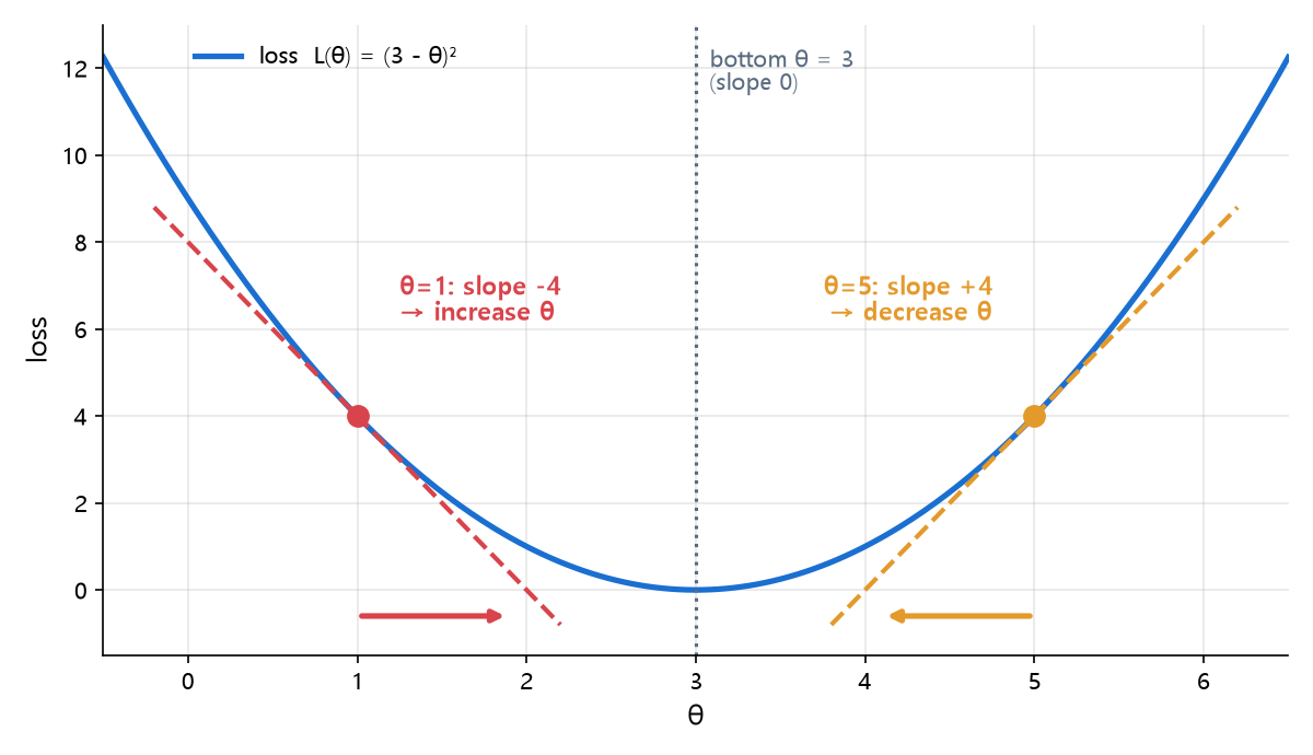
- At θ = 1 the tangent slope is −4. The loss goes down to the right, so θ should increase.
- At θ = 5 the tangent slope is +4. The loss goes up to the right, so θ should decrease.
- At θ = 3 (the bottom) the slope is 0, so there is no reason to move.
In both cases, moving opposite to the sign of the slope brings θ closer to the bottom. That is the gradient descent rule:
θ ← θ − α · dL/dθThe minus sign means “the opposite direction” and the learning rate α means “how far”. All that is left is to find dL/dθ.
Step 2: find the derivative
The loss is L = (y − θx)². Here are two ways to differentiate it; both give the same answer.
Method A: expand, then differentiate (no chain rule)
Expanding the square gives an ordinary quadratic in θ.
L = y² − 2xyθ + x²θ²Differentiating with respect to θ, y² has no θ and becomes 0, −2xyθ becomes −2xy, and x²θ² becomes 2x²θ.
dL/dθ = −2xy + 2x²θ
      = −2x(y − θx)
      = −2x(y − ŷ)
Method B: the chain rule
Let the error be e = y − θx, so L = e². Differentiate the outer function (the square) and the inner function (the error) separately, then multiply.
dL/de = 2e          ← derivative of the square
de/dθ = −x          ← y is a constant; −θx differentiates to −x
dL/dθ = dL/de × de/dθ = 2e × (−x) = −2x(y − ŷ)
Method A is easier here, but as models grow it quickly becomes impractical to expand the whole formula. Method B is what scales, and applying it across a whole computational graph is backpropagation, the topic of part 4.
Step 3: plug it in and the update rule appears
Put the derivative from step 2 into the rule from step 1.
θ ← θ − α · (−2x(y − ŷ))
  = θ + 2αx(y − ŷ)
That is the line we took on trust in part 1. It reads in three pieces:
| Piece | Meaning |
|---|---|
y − ŷ (error) | Prediction too small → positive → θ grows. Too large → negative → θ shrinks. Exact → 0 → θ stops |
x (input) | A larger input changes the prediction more per unit of θ, so the correction is larger |
2α | The step size; the 2 comes from differentiating the square |
Checking it in C++ and Python
Let us check the derived slope with numerical differentiation. Nudge θ up and down by a tiny amount (h = 0.00001) and divide the change in loss by 2h; that estimates the slope at that point without any formula. If the two numbers match, the derivation is right.
C++ (C++17, no external libraries)
#include <cstdio>
#include <initializer_list>

double Loss(double th, double x, double y) { return (y - th * x) * (y - th * x); }

double Grad(double th, double x, double y) { return -2.0 * x * (y - th * x); }   // derived by hand

double NumericGrad(double th, double x, double y, double h = 1e-5) {            // numerical check
    return (Loss(th + h, x, y) - Loss(th - h, x, y)) / (2.0 * h);
}

double TrainSingleSample(int iterations, double lr, double x, double y, double th = 0.1) {
    for (int it = 0; it < iterations; ++it) {
        const double pred = th * x;                       // 1) predict
        th = th - lr * (-2.0 * x * (y - pred));           // 2) θ ← θ − α · dL/dθ
    }
    return th;
}

int main() {
    std::printf("x=1, th=1: grad %.6f, numeric %.6fn", Grad(1, 1, 3), NumericGrad(1, 1, 3));
    std::printf("x=2, th=1: grad %.6f, numeric %.6fn", Grad(1, 2, 6), NumericGrad(1, 2, 6));
    std::printf("x=1, th=5: grad %.6f, numeric %.6fn", Grad(5, 1, 3), NumericGrad(5, 1, 3));
    for (double x : {0.5, 1.0, 2.0})
        std::printf("x=%.1f: th after 20 updates = %.5fn", x, TrainSingleSample(20, 0.1, x, 3 * x));
}
Python (standard library only)
def loss(th, x, y):
    return (y - th * x) ** 2

def grad(th, x, y):                          # derived by hand
    return -2 * x * (y - th * x)

def numeric_grad(th, x, y, h=1e-5):          # numerical check
    return (loss(th + h, x, y) - loss(th - h, x, y)) / (2 * h)

def train_single_sample(iterations, lr, x, y, th=0.1):
    for _ in range(iterations):
        pred = th * x                         # 1) predict
        th = th - lr * (-2 * x * (y - pred))  # 2) θ ← θ − α · dL/dθ
    return th

print(f"x=1, th=1: grad {grad(1, 1, 3):.6f}, numeric {numeric_grad(1, 1, 3):.6f}")
print(f"x=2, th=1: grad {grad(1, 2, 6):.6f}, numeric {numeric_grad(1, 2, 6):.6f}")
print(f"x=1, th=5: grad {grad(5, 1, 3):.6f}, numeric {numeric_grad(5, 1, 3):.6f}")
for x in [0.5, 1.0, 2.0]:
    print(f"x={x:.1f}: th after 20 updates = {train_single_sample(20, 0.1, x, 3 * x):.5f}")
This code uses no random numbers, so both languages print exactly the same thing.
Output
x=1, th=1: grad -4.000000, numeric -4.000000
x=2, th=1: grad -16.000000, numeric -16.000000
x=1, th=5: grad 4.000000, numeric 4.000000
x=0.5: th after 20 updates = 1.96039
x=1.0: th after 20 updates = 2.96657
x=2.0: th after 20 updates = 3.00000
At all three points the derived slope and the numerical estimate agree to six decimal places, including the −4 and +4 from the chart. The derivative the update rule is built on is correct.
Why not use numerical differentiation for training? With one parameter it would be fine. With a million parameters you would recompute the loss millions of times per update, which is far too slow. So training uses the derived formula (or backpropagation), and numerical differentiation is kept as a check that your derivative is right.
Same learning rate, larger x, faster learning
The last three lines of the output train three samples whose answer is 3 (x = 0.5, 1, 2), each with learning rate 0.1 for 20 updates. The results differ a lot.
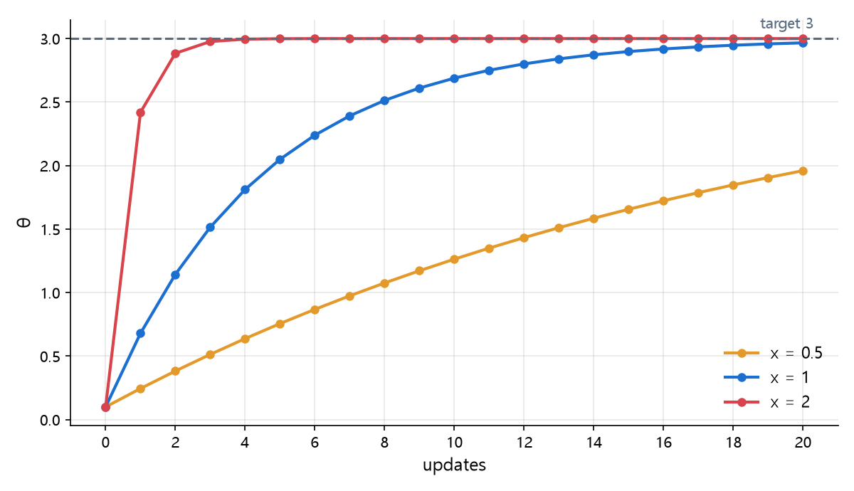
| Input x | θ after 1 update | θ after 20 updates | Factor on the remaining distance per update |
|---|---|---|---|
| 0.5 | 0.245 | 1.96039 | 0.95 |
| 1 | 0.68 | 2.96657 | 0.8 |
| 2 | 2.42 | 3.00000 | 0.2 |
In the update rule θ ← θ + 2αx(y − ŷ), we have y − ŷ = x(3 − θ), so every update multiplies the remaining distance 3 − θ by (1 − 2x²α). Doubling x makes x² four times larger, so with x = 2 the remaining distance drops to 0.2 of itself each step and θ is almost at 3 after four updates. With x = 0.5 it only shrinks to 0.95 each step, and after 20 updates θ has covered only about two thirds of the way.
So the right learning rate depends on the size of the inputs. A large x turns the same learning rate into a big step, and a step that is too big jumps past the bottom. What happens when (1 − 2x²α) turns negative or drops below −1 is the topic of the next part.
Common sources of confusion
Dropping the minus sign
The rule is θ − α·slope, and the slope itself carries a minus sign, so the update ends up with a plus. Get one sign wrong in code and θ walks away from the bottom while the loss keeps growing. If the loss rises as you train, check the signs first.
The 2 can go, but then the learning rate means something else
You can drop the 2 and write θ + αx(y − ŷ), and training still works. But then the same α gives a step half as large. When you copy a learning rate from another source, this difference alone can change the result.
Slowing down near the bottom is normal
The error y − ŷ is part of the slope, so the steps shrink by themselves as θ approaches the answer. That is why θ crept toward 3 at the end of the chart in part 1.
Deep learning gradient descent in summary
- The gradient descent rule is
θ ← θ − α · dL/dθ; moving opposite to the sign of the slope brings you closer to the bottom. - Differentiating
L = (y − θx)²givesdL/dθ = −2x(y − ŷ), and plugging it in givesθ ← θ + 2αx(y − ŷ). - Numerical differentiation confirmed the derived slope exactly at three points.
- Each update multiplies the remaining distance by
(1 − 2x²α), so with the same learning rate a larger x learns faster.
The next part uses (1 − 2x²α) to find, with real numbers, when a larger learning rate starts to oscillate and when it diverges.
Try it yourself
- Change the
-inth = th - lr * (...)to+and run it. θ moves away from 3. - Increase
hinNumericGradfrom1e-5to1.0. Because this loss is quadratic, the central difference is still exact. Then change the loss to something like(y − θx)⁴and watch the numerical estimate drift once h is large.