Why a larger deep learning learning rate oscillates and then diverges, explained with one multiplier, (1 − 2x²α), and checked with C++ and Python runs.
The first wall you hit when training a model is the learning rate. Too small and nothing happens for hours; a little larger and the loss suddenly explodes. This part derives exactly where the deep learning learning rate switches between “slow”, “oscillating”, and “diverging”, using a single number, and checks it with real runs.
Series guide: See all 11 parts and what is already published in the Deep Learning Math in C++ roadmap. This part continues from part 2: deriving the update rule.
The short answer
With a single sample, each update multiplies the remaining distance to the answer by f = 1 − 2x²α. If 0 < f < 1 training converges smoothly, if −1 < f < 0 it overshoots back and forth while converging, and if |f| > 1 every update moves further away and training diverges. The safe upper limit is therefore 1/x², and the larger the input x, the smaller the learning rate must be.
What this post answers
- Why a large learning rate overshoots the bottom, and where divergence starts
- How to compute the boundaries between converging, oscillating, and diverging
- Why the same learning rate can be safe for one x and dangerous for another
- How to judge the learning rate when there are several samples
New terms in this part
| Term | Meaning |
|---|---|
| Convergence | Parameters getting closer and closer to one value (here, the answer 3) as updates repeat |
| Oscillation | The parameter repeatedly jumping past the answer and coming back; if the swings shrink, it still converges |
| Divergence | Each update moves further from the answer until the numbers blow up |
Multiplier f | The number the “remaining distance to the answer” is multiplied by on each update; here 1 − 2x²α |
| Hyperparameter | A value set by a person rather than learned: learning rate, number of epochs, batch size, and so on |
One number multiplies the remaining distance
Start from the update rule derived in part 2. If the data follow y = 3x, then y − θx = x(3 − θ), so:
θ_new = θ + 2αx(y − θx)
      = θ + 2αx²(3 − θ)
Subtracting the answer 3 from both sides makes it clean:
θ_new − 3 = (1 − 2x²α)(θ − 3)In words: remaining distance after the update = multiplier f × remaining distance before it. f depends only on x and α, not on θ, so after k updates on the same sample the remaining distance is exactly f to the power k times the starting distance. You can predict how training will go before running a single update.
Five cases decided by f
| Multiplier f | Learning rate range (for x = 1) | Result |
|---|---|---|
0 < f < 1 | α < 1/(2x²) (below 0.5) | Approaches from one side: smooth convergence |
f = 0 | α = 1/(2x²) (exactly 0.5) | Reaches the answer in one step |
−1 < f < 0 | 1/(2x²) < α < 1/x² (0.5 to 1) | Jumps across the answer: oscillating convergence |
f = −1 | α = 1/x² (exactly 1) | Bounces between two values forever |
f < −1 | α > 1/x² (above 1) | Each jump lands further away: divergence |
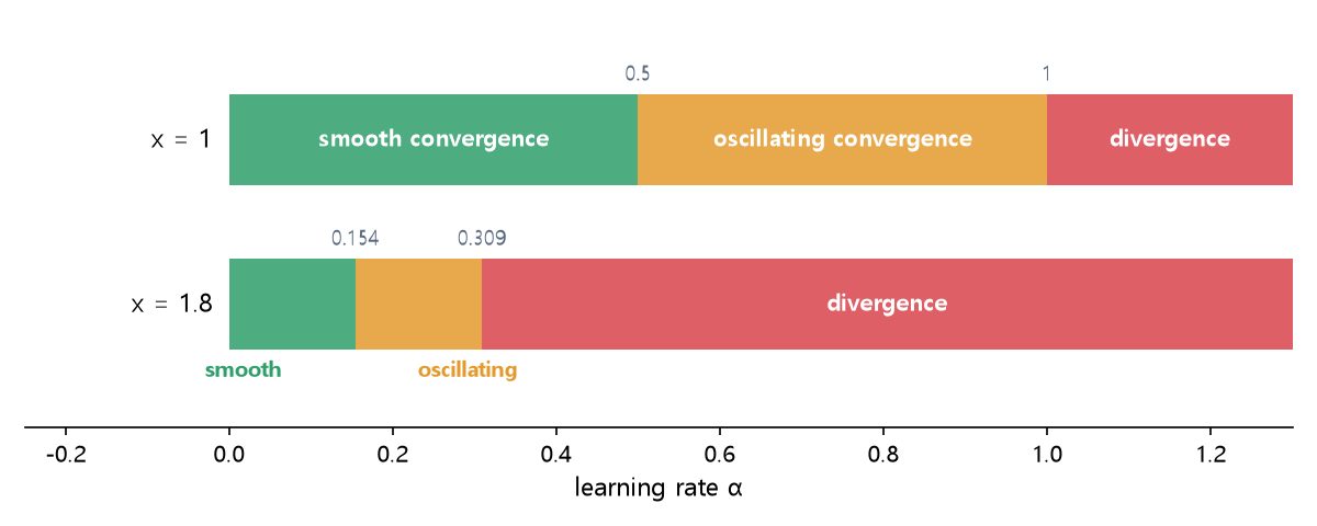
What matters is that both boundaries, 1/(2x²) and 1/x², contain x². With x = 1 even a learning rate of 0.9 converges, but with x = 1.8 the boundaries shrink to 0.154 and 0.309, and 0.3 is already on the edge of divergence.
Following an oscillation by hand
With x = 1 and learning rate 0.8, f = 1 − 2 × 1 × 0.8 = −0.6. Starting from 0.1, here are three updates:
| Update | θ | Distance to answer (θ − 3) | Times the previous distance |
|---|---|---|---|
| 0 | 0.1 | −2.9 | |
| 1 | 4.74 | +1.74 | −0.6 |
| 2 | 1.956 | −1.044 | −0.6 |
| 3 | 3.6264 | +0.6264 | −0.6 |
The sign of the distance flips every time: θ jumps past 3 to 4.74, then back below 3 to 1.956, and so on. But the size shrinks by 0.6 each time, so it still converges to 3.
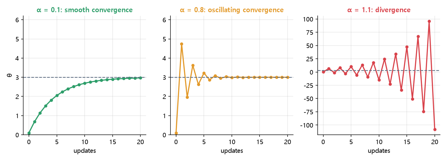
At a learning rate of 1.1, f = −1.2. It is the same kind of oscillation, but each jump lands 1.2 times further away, and after 20 updates θ has shot out to −108.
Checking it in C++ and Python
Three experiments in one run:
- Fix x = 1 and change only the learning rate
- Fix the learning rate at 0.3 and change only x
- Train three samples (x = 0.5, 1, 1.7) in order for 10 epochs
C++ (C++17, no external libraries)
#include <cstdio>
#include <initializer_list>
#include <utility>
#include <vector>

double TrainSingleSample(int iterations, double lr, double x, double y, double th = 0.1) {
    for (int it = 0; it < iterations; ++it)
        th = th + 2.0 * x * lr * (y - th * x);           // update rule from part 2
    return th;
}

double TrainEpochs(const std::vector<std::pair<double, double>>& samples, double lr, int epochs,
                   double th = 0.1) {
    for (int epoch = 0; epoch < epochs; ++epoch)
        for (const auto& [x, y] : samples)               // one sample at a time, in order
            th = th + 2.0 * x * lr * (y - th * x);
    return th;
}

int main() {
    // Experiment 1: one sample (x=1, y=3), change only the learning rate, 20 updates
    const double x1 = 1.0;
    for (double lr : {0.1, 0.5, 0.8, 1.0, 1.1}) {
        const double factor = 1.0 - 2.0 * x1 * x1 * lr;  // multiplier on the remaining distance
        std::printf("lr=%-4g factor=%+.2f  th after 20 = %.5fn", lr, factor,
                    TrainSingleSample(20, lr, x1, 3 * x1));
    }

    // Experiment 2: same learning rate 0.3, change only x
    for (double x : {0.5, 1.0, 1.8}) {
        const double factor = 1.0 - 2.0 * x * x * 0.3;
        std::printf("x=%-4g factor=%+.3f  th after 20 = %.5fn", x, factor,
                    TrainSingleSample(20, 0.3, x, 3 * x));
    }

    // Experiment 3: three samples (x=0.5, 1, 1.7) in order for 10 epochs
    const std::vector<std::pair<double, double>> samples = {{0.5, 1.5}, {1.0, 3.0}, {1.7, 5.1}};
    for (double lr : {0.01, 0.1, 0.6, 1.0})
        std::printf("3 samples, lr=%-4g  th after 10 epochs = %.5fn", lr, TrainEpochs(samples, lr, 10));
}
Python (standard library only)
def train_single_sample(iterations, lr, x, y, th=0.1):
    for _ in range(iterations):
        th = th + 2 * x * lr * (y - th * x)       # update rule from part 2
    return th

def train_epochs(samples, lr, epochs, th=0.1):
    for _ in range(epochs):
        for x, y in samples:                       # one sample at a time, in order
            th = th + 2 * x * lr * (y - th * x)
    return th

# Experiment 1: one sample (x=1, y=3), change only the learning rate, 20 updates
x1 = 1.0
for lr in [0.1, 0.5, 0.8, 1.0, 1.1]:
    factor = 1 - 2 * x1 * x1 * lr                  # multiplier on the remaining distance
    print(f"lr={lr:<4g} factor={factor:+.2f}  th after 20 = {train_single_sample(20, lr, x1, 3 * x1):.5f}")

# Experiment 2: same learning rate 0.3, change only x
for x in [0.5, 1.0, 1.8]:
    factor = 1 - 2 * x * x * 0.3
    print(f"x={x:<4g} factor={factor:+.3f}  th after 20 = {train_single_sample(20, 0.3, x, 3 * x):.5f}")

# Experiment 3: three samples (x=0.5, 1, 1.7) in order for 10 epochs
samples = [(0.5, 1.5), (1.0, 3.0), (1.7, 5.1)]
for lr in [0.01, 0.1, 0.6, 1.0]:
    print(f"3 samples, lr={lr:<4g}  th after 10 epochs = {train_epochs(samples, lr, 10):.5f}")
Output
lr=0.1  factor=+0.80  th after 20 = 2.96657
lr=0.5  factor=+0.00  th after 20 = 3.00000
lr=0.8  factor=-0.60  th after 20 = 2.99989
lr=1    factor=-1.00  th after 20 = 0.10000
lr=1.1  factor=-1.20  th after 20 = -108.17904
x=0.5  factor=+0.850  th after 20 = 2.88760
x=1    factor=+0.400  th after 20 = 3.00000
x=1.8  factor=-0.944  th after 20 = 2.08412
3 samples, lr=0.01  th after 10 epochs = 1.75743
3 samples, lr=0.1   th after 10 epochs = 2.99997
3 samples, lr=0.6   th after 10 epochs = 2.99993
3 samples, lr=1     th after 10 epochs = -17632.06267
Reading the results
Experiment 1: changing only the learning rate
- 0.1 is safe, but after 20 updates it is still at 2.96657, short of the answer.
- 0.5 gives
f = 0, so the very first update lands exactly on 3. - 0.8 oscillates yet still gets to 2.99989. Oscillation alone does not make a learning rate bad.
- 1.0 gives
f = −1, so θ bounces between 0.1 and 5.9 forever. After 20 updates (an even number) it is back at its starting value of 0.1. - 1.1 shot out to −108. With more updates the numbers keep growing until they exceed what the computer can represent.
Experiment 2: changing only x
The same learning rate of 0.3 gives completely different results. For x = 1, f = 0.4 and θ reaches 3 within 20 updates. For x = 0.5, f = 0.85 and θ creeps to 2.88760. For x = 1.8, f = −0.944: technically inside the converging range, but the distance shrinks by only 5.6% per update, so after 20 updates θ is still swinging widely at 2.08412.
A learning rate is not large or small on its own. You have to judge it together with the size of x.
Experiment 3: several samples
With several samples, each sample has its own multiplier. Using the three samples once per epoch multiplies the remaining distance by the product of the three multipliers.
| Learning rate | f for x = 0.5 | f for x = 1 | f for x = 1.7 | Multiplier per epoch (product) | θ after 10 epochs |
|---|---|---|---|---|---|
| 0.01 | +0.995 | +0.980 | +0.942 | +0.919 | 1.75743 |
| 0.1 | +0.950 | +0.800 | +0.422 | +0.321 | 2.99997 |
| 0.6 | +0.700 | −0.200 | −2.468 | +0.346 | 2.99993 |
| 1.0 | +0.500 | −1.000 | −4.780 | +2.390 | −17632 |
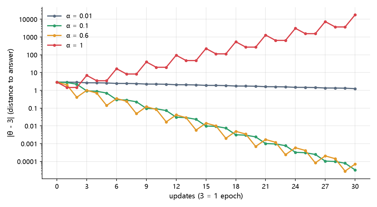
Learning rate 0.6 is an interesting case. On its own, the x = 1.7 sample has f = −2.468 and should diverge, but the other two samples shrink the distance enough that the whole epoch still multiplies it by 0.346. That only works because all three samples in this experiment share exactly the same answer, 3. With noisy real data, one sample with a large x can kick θ far away and destabilize training, so treat the limit for the largest x, 1/x_max² (here 1/1.7² ≈ 0.35), as the safe line. The epoch multiplier 0.346 in the table happens to look similar, but it is a different quantity.
Choosing a learning rate in practice
You can rarely compute the exact limit with a formula, but the principle carries over.
- Look at the size of the inputs first. Inputs in the tens or hundreds need a very small learning rate.
- Start small and grow by 10×. Try 0.0001 → 0.001 → 0.01 → 0.1 with short runs and compare.
- Watch the training curve. If the loss swings up and down, lower the learning rate; if the numbers explode, lower it a lot; if it falls too slowly, raise it.
- Matching input sizes is another option. Instead of shrinking the learning rate, rescale the inputs to a similar size so a normal learning rate trains stably. That is feature scaling, the topic of part 10.
Common sources of confusion
An oscillating learning rate is not always bad
In experiment 1, 0.8 oscillated yet got closer to the answer than 0.1. A smaller |f| is faster, and 0.8 (|f| = 0.6) beats 0.1 (|f| = 0.8). The problem is not oscillation itself but |f| approaching or exceeding 1.
A flat loss is not always a learning rate that is too small
With learning rate 1.0, f = −1: θ bounces between two values and the loss repeats the same value. On a chart it looks as if training stopped, but the learning rate is actually too large. Check whether θ keeps alternating between two values on either side of the answer.
A learning rate that worked elsewhere can be dangerous here
A learning rate that worked in another tutorial can diverge on inputs of a different size. In experiment 2, 0.3 reached the answer within 20 updates for x = 1 but sat on the edge of divergence for x = 1.8.
Deep learning learning rate in summary
- With one sample, each update multiplies the remaining distance by
f = 1 − 2x²α. |f| < 1converges (oscillating when negative) and|f| > 1diverges; the safe limit isα < 1/x².- The limit is inversely proportional to x², so larger inputs need a smaller learning rate.
- With several samples, the multiplier per epoch is the product of the per-sample multipliers, but in practice the limit for the largest x is the safe line.
The next part looks at computational graphs and backpropagation with five node types, which compute the derivatives we have been deriving by hand, however long the formula gets.
Try it yourself
- Add a learning rate of 0.99 to experiment 1. With
f = −0.98it still converges, but after 20 updates θ is only at about 1.06, with roughly two thirds of the starting distance left. Compare it with learning rate 0.01, which has the same|f| = 0.98and moves at the same speed. - Reorder experiment 3 so that
{1.7, 5.1}comes first. Check whether θ after 10 epochs changes, and explain why using the product of the multipliers.