Understand deep learning backpropagation through five node types (add, subtract, multiply, square, mean), follow a forward and backward pass by hand, and confirm it in C++ and Python.
In part 2 we differentiated the loss (y − θx)² by hand and got the gradient −2x(y − ŷ). That worked because the formula was short. In a network with dozens of layers, even writing the loss as one formula is hard. Yet deep learning frameworks compute gradients for any model automatically. How they do it is the topic of this part: deep learning backpropagation.
Series guide: See all 11 parts and what is already published in the Deep Learning Math in C++ roadmap.
The short answer
Backpropagation splits a long formula into small nodes that each do one operation, then walks backwards from the output to the inputs, passing along “the gradient that came from behind × this node’s local derivative”. Each node only needs to know the derivative of its own operation, so the same rule computes gradients no matter how long the formula is.
What this post answers
- What a computational graph is and why formulas are split into nodes
- What the forward pass and the backward pass each compute
- How add, subtract, multiply, square, and mean nodes pass gradients
- Whether gradients from nodes really match the hand-derived formula
New terms in this part
| Term | Meaning |
|---|---|
| Computational graph | A drawing of a formula as operation nodes connected by arrows that carry values |
| Node | A unit that performs one operation, such as addition or multiplication |
| Forward pass | Computing values from inputs to output; this produces the prediction and the loss |
| Backward pass (backpropagation) | Passing gradients from the output back to the inputs; this produces each parameter’s gradient |
| Local gradient | The derivative of a node’s output with respect to its own inputs, computed inside the node |
| Upstream gradient | The gradient arriving from the node behind (closer to the output), usually called dz in code |
Splitting the formula into nodes
The loss L = (y − θx)² is made of three operations. Naming each step:
z1 = θ × x        ← multiply node (prediction)
z2 = y − z1       ← subtract node (error)
L  = z2²          ← square node (loss)
Each line is a single, simple operation. Connect them with arrows and you have a computational graph. Let us push the numbers θ = 1, x = 2, y = 6 through it, the same sample whose gradient was −16 in part 2.
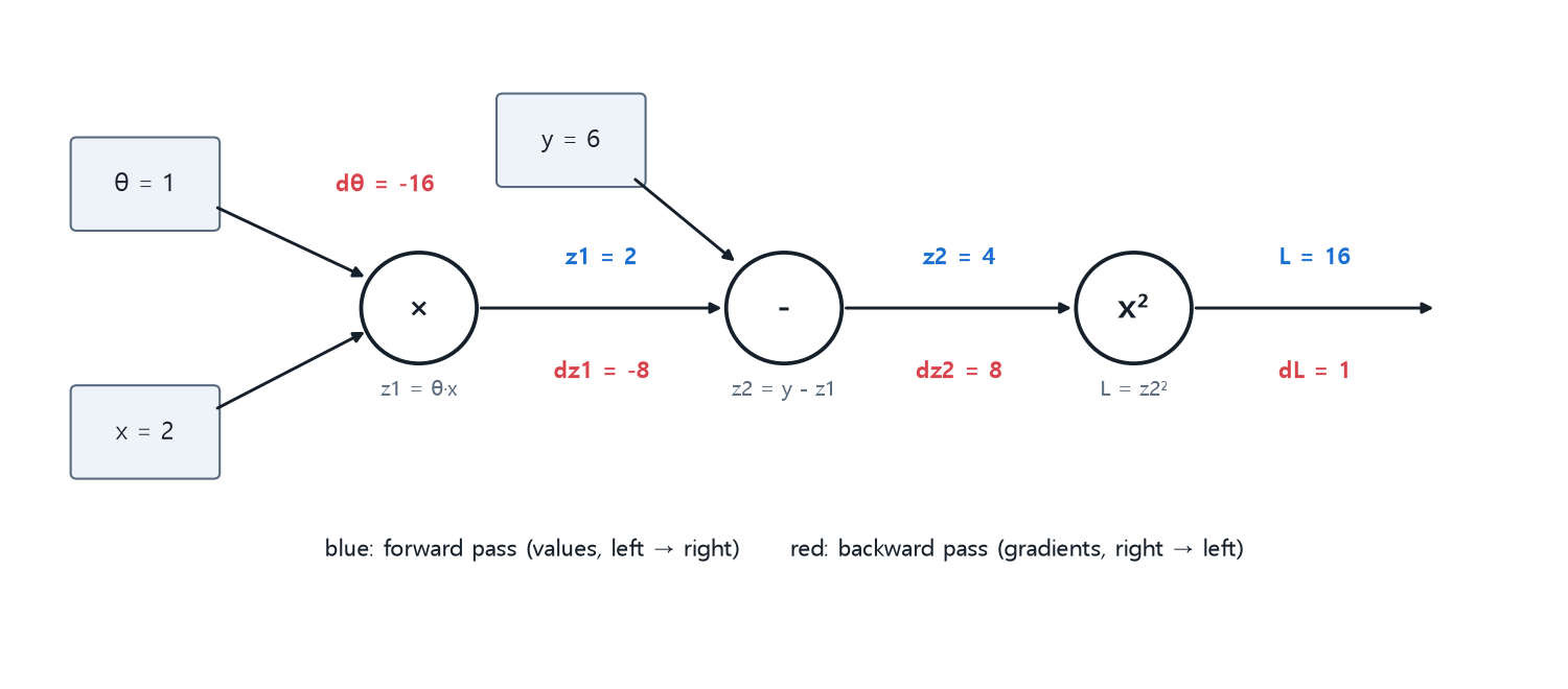
Forward pass: values from left to right
z1 = θ × x  = 1 × 2 = 2
z2 = y − z1 = 6 − 2 = 4
L  = z2²    = 4²    = 16
This is the same predict-and-measure computation we have used since part 1. The difference is that each node remembers its inputs, because the backward pass needs them.
Backward pass: gradients from right to left
The backward pass starts at the end with dL/dL = 1, the obvious fact that changing L changes L by the same amount. Then each node multiplies the incoming gradient by its own local derivative and passes the result forward.
square node:    local derivative 2·z2 = 8      →  dz2 = 1 × 8    = 8
subtract node:  local derivative for z1 is −1  →  dz1 = 8 × (−1) = −8
multiply node:  local derivative for θ is x = 2 →  dθ  = −8 × 2   = −16
The result dθ = −16 matches the formula −2x(y − ŷ) = −2 × 2 × (6 − 2) from part 2. That is the chain rule: method B in part 2 multiplied the outer and inner derivatives, and here we simply do the same thing node by node.
Local derivatives of the five nodes
All the linear regression computations in this series can be written as combinations of the five nodes below. Real neural networks also need nodes such as activation functions, but the principle is the same: each node only needs the derivative of its own operation.
| Node | Forward | Backward (what it returns given dz) | Remember |
|---|---|---|---|
| Add | z = x + y | dz to x, dz to y | Copies the gradient |
| Subtract | z = x − y | dz to x, −dz to y | Only the subtracted side flips sign |
| Multiply | z = x × y | dz × y to x, dz × x to y | Multiplies by the other input |
| Square | z = x² | dz × 2x | Needs the input x |
| Mean | z = (x₁ + … + xₙ) / n | dz / n to every xᵢ | Splits the gradient evenly n ways |
The multiply and square nodes need the inputs from the forward pass, which is why nodes store their inputs. This storage is also one reason deep learning frameworks use so much memory during training.
Here are the nodes as I implemented them in C++, with numbers plugged in: x = 2, y = 3 for add, subtract, and multiply; x = 3 for square; [1, 2, 3, 4, 5] for mean; and an incoming gradient of dz = 2 in every case.
| Node | Forward result z | Backward result |
|---|---|---|
| Add | 5 | (2, 2) |
| Subtract | −1 | (2, −2) |
| Multiply | 6 | (6, 4) |
| Square | 9 | 12 |
| Mean | 3 | [0.4, 0.4, 0.4, 0.4, 0.4] |
This part’s model uses only multiply, subtract, and square. The mean node returns in part 6, which handles the loss of many samples at once, and the add node in part 7, which adds a bias.
Checking it in C++ and Python
We write the nodes as classes and check two things:
- With
θ = 1, x = 2, y = 6, one forward and one backward pass match the hand calculation above - Training the three samples from part 3 (x = 0.5, 1, 1.7) with nodes gives the same result as the update rule from part 2
C++ (C++17, no external libraries)
#include <cmath>
#include <cstdio>
#include <utility>
#include <vector>

class MulNode {                                   // z = x * y
public:
    double Forward(double x, double y) {
        x_ = x; y_ = y;                           // keep the inputs for the backward pass
        return x * y;
    }
    std::pair<double, double> Backward(double dz) const {
        return {dz * y_, dz * x_};                // each side gets the other input
    }
private:
    double x_ = 0, y_ = 0;
};

class MinusNode {                                 // z = x - y
public:
    double Forward(double x, double y) { return x - y; }
    std::pair<double, double> Backward(double dz) const {
        return {dz, -dz};                         // the subtracted side flips sign
    }
};

class SquareNode {                                // z = x²
public:
    double Forward(double x) {
        x_ = x;
        return x * x;
    }
    double Backward(double dz) const { return dz * 2.0 * x_; }   // derivative of the square: 2x
private:
    double x_ = 0;
};

int main() {
    MulNode mul;
    MinusNode minus;
    SquareNode square;

    // 1) One sample (x=2, y=6, θ=1): one forward and one backward pass
    {
        const double th = 1.0, x = 2.0, y = 6.0;
        const double z1 = mul.Forward(th, x);     // forward: inputs → output
        const double z2 = minus.Forward(y, z1);
        const double l = square.Forward(z2);
        const double dz2 = square.Backward(1.0);  // backward: output → inputs (start from dL/dL = 1)
        const auto [dy, dz1] = minus.Backward(dz2);
        const auto [dth, dx] = mul.Backward(dz1);
        std::printf("forward : z1=%g, z2=%g, L=%gn", z1, z2, l);
        std::printf("backward: dz2=%g, dz1=%g, dth=%g  (formula -2x(y-pred) = %g)n",
                    dz2, dz1, dth, -2.0 * x * (y - th * x));
    }

    // 2) Train with nodes and with the part 2 update rule, then compare
    const std::vector<std::pair<double, double>> samples = {{0.5, 1.5}, {1.0, 3.0}, {1.7, 5.1}};
    double th_node = 0.1, th_formula = 0.1;
    const double lr = 0.1;
    for (int epoch = 0; epoch < 10; ++epoch) {
        for (const auto& [x, y] : samples) {
            const double z1 = mul.Forward(th_node, x);
            const double z2 = minus.Forward(y, z1);
            square.Forward(z2);
            const double dz2 = square.Backward(1.0);
            const double dz1 = minus.Backward(dz2).second;
            const double dth = mul.Backward(dz1).first;
            th_node = th_node - lr * dth;                                  // gradient from the nodes
            th_formula = th_formula + 2.0 * x * lr * (y - th_formula * x); // part 2 update rule
        }
    }
    std::printf("nodes  : th = %.5fn", th_node);
    std::printf("formula: th = %.5fn", th_formula);
    std::printf("diff   : %.1en", std::fabs(th_node - th_formula));
}
Python (standard library only)
class MulNode:                              # z = x * y
    def forward(self, x, y):
        self.x, self.y = x, y               # keep the inputs for the backward pass
        return x * y
    def backward(self, dz):
        return dz * self.y, dz * self.x     # each side gets the other input

class MinusNode:                            # z = x - y
    def forward(self, x, y):
        return x - y
    def backward(self, dz):
        return dz, -dz                      # the subtracted side flips sign

class SquareNode:                           # z = x²
    def forward(self, x):
        self.x = x
        return x * x
    def backward(self, dz):
        return dz * 2 * self.x              # derivative of the square: 2x

mul, minus, square = MulNode(), MinusNode(), SquareNode()

# 1) One sample (x=2, y=6, θ=1): one forward and one backward pass
th, x, y = 1.0, 2.0, 6.0
z1 = mul.forward(th, x)                     # forward: inputs → output
z2 = minus.forward(y, z1)
l = square.forward(z2)
dz2 = square.backward(1.0)                  # backward: output → inputs (start from dL/dL = 1)
dy, dz1 = minus.backward(dz2)
dth, dx = mul.backward(dz1)
print(f"forward : z1={z1:g}, z2={z2:g}, L={l:g}")
print(f"backward: dz2={dz2:g}, dz1={dz1:g}, dth={dth:g}  (formula -2x(y-pred) = {-2 * x * (y - th * x):g})")

# 2) Train with nodes and with the part 2 update rule, then compare
samples = [(0.5, 1.5), (1.0, 3.0), (1.7, 5.1)]
th_node, th_formula, lr = 0.1, 0.1, 0.1
for epoch in range(10):
    for x, y in samples:
        z1 = mul.forward(th_node, x)
        z2 = minus.forward(y, z1)
        l = square.forward(z2)
        dz2 = square.backward(1.0)
        dy, dz1 = minus.backward(dz2)
        dth, dx = mul.backward(dz1)
        th_node = th_node - lr * dth                              # gradient from the nodes
        th_formula = th_formula + 2 * x * lr * (y - th_formula * x)  # part 2 update rule
print(f"nodes  : th = {th_node:.5f}")
print(f"formula: th = {th_formula:.5f}")
print(f"diff   : {abs(th_node - th_formula):.1e}")
Output
forward : z1=2, z2=4, L=16
backward: dz2=8, dz1=-8, dth=-16  (formula -2x(y-pred) = -16)
nodes  : th = 2.99997
formula: th = 2.99997
diff   : 0.0e+00
The first two lines repeat the chart and the hand calculation. The last three show that θ trained with node gradients and θ trained with the part 2 formula stay identical to the end. They also match part 3’s result for the same setup (learning rate 0.1, 10 epochs): 2.99997.
In the C++ code, const auto [dy, dz1] = ... is a C++17 structured binding, the equivalent of Python’s dy, dz1 = .... Each node returns the gradients for both of its inputs as a pair, but this model never uses dy or dx: the answer y and the input x are not values that training changes.
Why bother splitting into nodes
For this example, the one-line formula is much shorter than the node code. There are still three reasons to use nodes:
- Nodes survive model changes. When part 7 adds a bias, we just insert one add node. With the formula approach you would redo the derivative from scratch.
- Each node can be tested on its own. Check each node with numbers, like the five-node table above, and you can trust the larger model built from them.
- This is how frameworks work. PyTorch and TensorFlow record the formula you write as a graph of nodes, and when you ask for gradients (
loss.backward()in PyTorch,GradientTapein TensorFlow) they pass gradients back in the same order as this post.
Common sources of confusion
Backpropagation computes gradients; it does not train
Backpropagation stops once it has dθ. Changing θ is the job of the next line, gradient descent: θ ← θ − α · dθ. “Training with backpropagation” is shorthand for “computing gradients with backpropagation and updating with gradient descent”.
The multiply node multiplies by the other input
Differentiating z = θ × x with respect to θ leaves x, so θ receives dz × x. A common first-implementation bug is writing dz × θ, which breaks the gradient completely.
No forward pass, no backward pass
The multiply and square nodes need the inputs saved during the forward pass. That is why one training step always runs forward pass → backward pass → update.
Deep learning backpropagation in summary
- A computational graph splits a formula into nodes that each do one operation.
- The forward pass computes values from inputs to output; the backward pass passes “incoming gradient × local derivative” from the output back to the inputs.
- Add copies, subtract flips one side, multiply uses the other input, square multiplies by 2x, and mean splits evenly n ways.
- Gradients from nodes and the hand-derived formula produce exactly the same training result.
The next part looks at training from the data side: why the same learning rate works for one input distribution and fails for another.
Try it yourself
- Deliberately change the backward of
MulNodeto{dz * x_, dz * y_}(each side gets its own input instead of the other one) and run it.dthcomes out wrong, −8 instead of −16. Yet training still lands on 3.00000. In this data x and θ are both positive, so the wrong gradient still points in the right direction. A wrong gradient can look like it trains fine, which is why you should test each node with numbers, like the five-node table, instead of only checking the final result. - Write your own
PlusNode: forward returnsx + y, backward returns{dz, dz}. Part 7 uses exactly this node to add a bias.